The paths, or rather, the orbits of the galaxies are given in a somewhat different manner in the AVP compared with equation (3.2); namely P-89
where the superscript ![]() represents the spatial dimensions;
represents the spatial dimensions;
![]() (not to be confused with the parameter from Hamilton's principle).
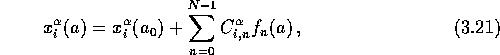
By comparing equation (3.2) with equation (3.21), one notice
a few distinct differences--modifications of Hamilton's principle introduced by
P-89. Firstly, the scale factor is used as a measure of time, which is justified
due to the close link between time and scale factor. This is common practise in cosmology.
Secondly, the first term on the right hand side in (3.2) is time
dependent, while the corresponding term in (3.21) is not. The result of this
alteration is that the term no longer represents the correct path in the AVP as it did
in equation (3.2), but rather the present positions of the particles.
Thirdly, the orbits are parameterized in the AVP picture; i.e. they are built up by the
sum in the second term of equation (3.21). The
(not to be confused with the parameter from Hamilton's principle).
By comparing equation (3.2) with equation (3.21), one notice
a few distinct differences--modifications of Hamilton's principle introduced by
P-89. Firstly, the scale factor is used as a measure of time, which is justified
due to the close link between time and scale factor. This is common practise in cosmology.
Secondly, the first term on the right hand side in (3.2) is time
dependent, while the corresponding term in (3.21) is not. The result of this
alteration is that the term no longer represents the correct path in the AVP as it did
in equation (3.2), but rather the present positions of the particles.
Thirdly, the orbits are parameterized in the AVP picture; i.e. they are built up by the
sum in the second term of equation (3.21). The ![]() used in Hamilton's
principle is in the AVP replaced by N coefficients,
used in Hamilton's
principle is in the AVP replaced by N coefficients, ![]() , and by summing
up the product of these coefficients and their respective functions
, and by summing
up the product of these coefficients and their respective functions ![]() , one gets
an estimate of the particle orbits.
, one gets
an estimate of the particle orbits.
What is similar, however, are the functions used in the second term of both equation
(3.2) and (3.21). The ![]() used in the AVP, often
referred to as trial functions, have some of the same characteristics as the
used in the AVP, often
referred to as trial functions, have some of the same characteristics as the ![]() function used in equation (3.2): they are both twice differentiable and
continuous in the interval of the action. But, when it comes to the constraints given at
the end-points, the two principles differ somewhat once again. While the
function used in equation (3.2): they are both twice differentiable and
continuous in the interval of the action. But, when it comes to the constraints given at
the end-points, the two principles differ somewhat once again. While the ![]() in
Hamilton's principle is forced to vanish at both end-points, the trial functions
in
Hamilton's principle is forced to vanish at both end-points, the trial functions
![]() only need to vanish at the end-point representing the present time. The
constraint at the other end-point, representing the initial time, is that the derivate
of
only need to vanish at the end-point representing the present time. The
constraint at the other end-point, representing the initial time, is that the derivate
of ![]() with respect to time vanishes. This is a result of the mixed boundary
condition introduced by P-89, as discussed in Section 3.1. More
details on these boundary conditions in the following subsection.
with respect to time vanishes. This is a result of the mixed boundary
condition introduced by P-89, as discussed in Section 3.1. More
details on these boundary conditions in the following subsection.
Now, let us take a closer look at the shape of these trial functions ![]() . The
choice of functions can be arbitrary, provided that they are complete enough to make a
fit of a gravitationally evolving density field between the two end-points; i.e. to
mimic the deformation of the path. In this thesis, two different types of trial
functions have been used; the fairly simple P-89,D-L,B-C
. The
choice of functions can be arbitrary, provided that they are complete enough to make a
fit of a gravitationally evolving density field between the two end-points; i.e. to
mimic the deformation of the path. In this thesis, two different types of trial
functions have been used; the fairly simple P-89,D-L,B-C
and the more complex Bernoulli distribution, P-90
where the expansion factor, a, is being normalized to unity at the present
time; ![]() . The type of trial functions has very little effect on the
solution. However, as pointed out by Gia, it does have an effect on the
computation of the solution, at least for systems involving a large number of particles,
say, thousands of objects. With such extensive systems, considerable computing time may
be saved by choosing a trial function that gives a rapid convergence of the series in
equation (3.21). Peebles made use of the trial functions in equation
(3.22) in his first paper dealing with the AVP P-89, but later used
the Bernoulli distribution just because of its ability to speed up the computation.
Other trial functions than (3.22) and (3.23) have also been used
in literature, e.g. Gia,S-B,Sch used a polynomial in the linear growth function,
D(t).
. The type of trial functions has very little effect on the
solution. However, as pointed out by Gia, it does have an effect on the
computation of the solution, at least for systems involving a large number of particles,
say, thousands of objects. With such extensive systems, considerable computing time may
be saved by choosing a trial function that gives a rapid convergence of the series in
equation (3.21). Peebles made use of the trial functions in equation
(3.22) in his first paper dealing with the AVP P-89, but later used
the Bernoulli distribution just because of its ability to speed up the computation.
Other trial functions than (3.22) and (3.23) have also been used
in literature, e.g. Gia,S-B,Sch used a polynomial in the linear growth function,
D(t).
Equation (3.21) is only correct for an infinitely large N, which, of course, is impossible to handle numerically. Therefore, the number of terms in the series has to be finite, resulting in a discrepancy between the true orbit and the orbit obtained by the AVP. This error is referred to as ``truncation error''. For N=5, the number of correct significant digits in the positions are two, while for N=15 it has improved to six. The choice of N is a tradeoff between computing time and accuracy, and figures in literature ranges from five up to about twenty.