In a perfectly homogeneous Friedmann-universe, comoving particles will have velocities solely determined by the Hubble law. By introducing inhomogeneities, as in the standard model, the Hubble flow will be perturbed, resulting in peculiar velocities of the particles. These velocities can give us valuable information about the underlying mass distribution, and vice versa.
A discussion of the velocity fields can be found in textbooks like P-93 and Pad.
The peculiar velocities of galaxies emerge from the linear theory discussed in Subsection (2.2.2). The linearized mass conservation equation in comoving coordinates is given by
where ![]() is the peculiar velocity and
is the peculiar velocity and ![]() is the
density contrast (
is the
density contrast ( ![]() ). The calculations are greatly simplified
by transferring this equation into Fourier space, where one can treat each wavelength
separately. The Fourier transform of the density contrast and the peculiar velocity are,
respectively:
). The calculations are greatly simplified
by transferring this equation into Fourier space, where one can treat each wavelength
separately. The Fourier transform of the density contrast and the peculiar velocity are,
respectively:
By inserting these two equations into equation (2.18), and rearranging somewhat, the resulting peculiar velocities are
(A term has been ignored since it decreases with time.)
![]() can be rewritten as
can be rewritten as
where ![]() . By combining
equation (2.22) and (2.21), one have an expression for
the relation between velocity and density
. By combining
equation (2.22) and (2.21), one have an expression for
the relation between velocity and density
The value of f(a) at the current epoch has been shown to be very well
approximated by the power law ![]() [for further details,
see][page 163]Pad. Using this value for f, one sees that the density parameter
can be estimated if the velocity field and the density field were observationally
determined. The problem is to get an accurate enough determination of the velocity
field, which involve distance determinations which are not based on redshift.
[for further details,
see][page 163]Pad. Using this value for f, one sees that the density parameter
can be estimated if the velocity field and the density field were observationally
determined. The problem is to get an accurate enough determination of the velocity
field, which involve distance determinations which are not based on redshift.
In the gravitational instability picture one assumes that it is gravity that makes the
perturbations grow. It is therefore natural to introduce the gravitational potential
instead of the density contrast ![]() . The linearized Poisson equation in
comoving coordinates is
. The linearized Poisson equation in
comoving coordinates is
where ![]() is the background density. Solving for the Fourier transform
density contrast gives
is the background density. Solving for the Fourier transform
density contrast gives
Inserting this into equation (2.23) results in an expression for the connection between the velocity field and the gravitational potential
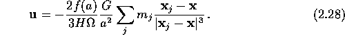
Equation (2.26) does not do us much good in the Fourier space--let us transfer it into real space:
For a particle system, with masses ![]() , this equation can be rewritten as
, this equation can be rewritten as
This equation show us that the velocity field is parallel and proportional to the peculiar acceleration, and then also to the gravitational force.